
Project Overview

This project developed a MATLAB-based finite element optimization tool for a linear static spring system. The benchmark model is a 7-node, 8-spring structural network fixed at both ends, with external loads applied at interior nodes. Although simplified, the model represents the same design logic used in mechanical systems such as supports, linkages, mounts, compliant structures, frames, and load-transfer paths.
The main engineering question was: given a limited stiffness budget, how should stiffness be distributed across the spring elements so the structure deforms less under load while still satisfying displacement limits? The tool starts with an initial spring design, assembles the finite element equations, solves for nodal displacements and reaction forces, evaluates compliance, and then uses constrained optimization to redistribute spring stiffness values.
Compliance was used as the main performance metric: θ = UᵀP
A higher compliance value means the structure is more flexible under load. A lower compliance value means the structure is stiffer and more efficient. In the benchmark case, the optimizer reduced compliance from 928.69 to 646.21, which is an improvement of about 30.4%. The final design used the full allowable stiffness budget of 31 and kept the maximum nodal displacement at the required limit of 12.
Methods
The finite element model treats each spring as a two-node element with a local stiffness matrix: Kₑ = kₑ [ 1 −1
−1 1 ]
Each element stiffness matrix is assembled into the global structural system. Because some nodes are fixed and others are free to move, the global system is partitioned into prescribed and free degrees of freedom: [ Kₚₚ Kₚf ] [ Uₚ ] = [ Pₚ ]
[ Kfₚ Kff ] [ Uf ] [ Pf ]
The unknown free displacements are solved using: Kff Uf = Pf − KfₚUₚ
Then reaction forces at constrained nodes are recovered using: Pₚ = KₚₚUₚ + KₚfUf
The design variables are the spring stiffness values: k = [k₁, k₂, k₃, k₄, k₅, k₆, k₇, k₈]
The optimization problem was formulated as: Minimize θ(k) = UᵀP
Subject to: Σᵢ₌₁⁸ kᵢ ≤ 31, |Uᵢ| ≤ 12, kᵢ ≥ 1 × 10⁻⁶
The total stiffness constraint represents a limited material, cost, or design-resource budget. The displacement constraint ensures that no node exceeds the allowable movement limit. The lower-bound stiffness constraint prevents numerical singularities while allowing springs to be effectively removed from the optimized load path.
Results and Interpretation
The initial stiffness vector was: k_initial = [2, 3, 3, 3, 4, 4, 5, 5]
The optimized stiffness vector was: k_optimized = [4.1646, 7.2747, 5.3302, 1.0×10⁻⁶, 5.5602, 3.1101, 1.0×10⁻⁶, 5.5602]
The initial and optimized compliance values were: θ_initial = 928.69,
θ_optimized = 646.21
The percent improvement was: Improvement = [(928.69 − 646.21) / 928.69] × 100 = 30.4%
The optimizer redistributed stiffness toward the spring elements that contributed most to load carrying.
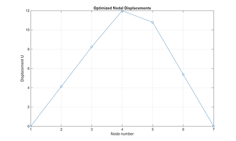
The optimized displacement vector was: U = [0, 4.1239, 8.2478, 12.0000, 10.7909, 5.3955, 0]
The final displacement profile satisfied the boundary conditions and reached the allowable displacement limit of 12.
The final stiffness budget was: Σᵢ₌₁⁸ kᵢ = 31
The optimizer used the full stiffness budget and reached the displacement limit, which is typical of a well-posed constrained structural optimization problem. Springs 2, 3, 5, and 8 retained relatively high stiffness values, showing that they were important to the main load path. Springs 4 and 7 were reduced to the lower bound, meaning they contributed little to the optimized response under this loading and support condition.
Initial versus optimized stiffness values show how the design shifted stiffness into the most effective load paths.


Validation, Skills, and Significance
A major part of the project involved debugging and validating the finite element and optimization workflow. The solver had to correctly assemble stiffness matrices, enforce boundary conditions, solve the partitioned system, recover reaction forces, update design variables, and generate usable outputs. Validation checks confirmed that fixed nodes retained prescribed displacement values, the stiffness matrix partitions had correct dimensions, reaction forces were recovered at constrained nodes, the optimized stiffness values satisfied the resource constraint, and the maximum displacement stayed within the allowable limit.
Optimization history showing convergence toward a feasible constrained design.
This project demonstrates finite element formulation, stiffness matrix assembly, boundary condition enforcement, matrix partitioning, static equilibrium solution, reaction force recovery, compliance-based optimization, constraint formulation, sensitivity analysis, MATLAB software development, numerical debugging, and engineering visualization.
The project connects finite element theory with practical mechanical design optimization. It shows how a structure can be modeled, analyzed, and improved through an automated computational workflow. By reducing compliance by approximately 30.4% while satisfying both stiffness and displacement constraints, the tool demonstrates how optimization can guide efficient stiffness allocation in mechanical systems.
